Continuous Probability Distributions

Continuous probability distributions describe the likelihood of a random variable taking on a value within a continuous range without gaps or interruptions. Continuous random variables have numerous applications across various fields. For example, they are used to model baseball batting averages, IQ scores, the duration of long-distance telephone calls, the lifespan of a computer chip, rates of return on investments, and SAT scores. Other examples include daily temperatures in a city, blood pressure readings, fuel efficiency of vehicles, reaction times in psychological tests, and time between arrivals of customers at a service center.

The field of reliability engineering relies heavily on continuous random variables to predict the longevity of products and systems, such as the time until failure of machinery or electronic components. Similarly, risk analysis across industries like finance, insurance, and environmental science depends on modeling continuous variables, such as stock market volatility, claim amounts in insurance policies, and river water levels during floods. These variables help professionals make informed decisions and manage uncertainty in real-world scenarios. This lesson focuses on two key continuous probability distributions: the uniform distribution and the normal distribution. These distributions are fundamental in statistical analysis later in the course (especially the normal distribution) so we must have a good understanding of how to work with each one.

The Uniform Distribution

In this lesson, we will explore how to calculate probabilities for uniform distributions. Uniform distributions are represented by a rectangular shape, where the total area under the curve equals 1 (or 100%). This establishes a direct relationship between probability and area. To find probabilities for uniform distributions, we calculate the area of the corresponding section of the rectangle, which is determined by the formula for area: length multiplied by width. Let’s apply this concept with some examples below.

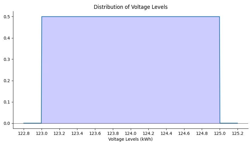
Example : Voltage Levels

Suppose a power company provides voltage levels uniformly distributed between 123.0 volts and 125.0 volts as pictured below in the image. What is the probability that a randomly selected voltage level is less than 123.7 volts?

Solution

Since we want a voltage less than 123.7 volts, we can identify this region on our probability distribution and shade it as we see in the image below:

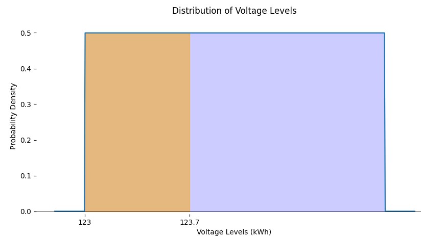
Now all we would need to do is find the area of this shaded region. Using a length of 0.7 and a width of 0.5, we know the total area of this highlighted piece from 123 volts to 123.7 volts would be \(0.7*0.5 = 0.35\). Since the area under the entire shape is equal to 1, this tells us that the probability is approximately 0.35 or 35% chance to select a voltage less than 123.7 volts.

Density Curves

This previous example introduced us to a graph of a density curve, which you will be seeing more and more of throughout the rest of this chapter.

When the graph of a continuous probability distribution (such as the rectangular "box" in the previous example) is drawn these are what are called density curves (or probability density functions, abbreviated as PDFs). Density curves always represent probabilities as areas under the curve. The total area under the curve is always equal to 1 for any density curve (this is true for both the uniform distribution observed in this section but also for the normal distributions we will see in the next section), indicating 100% certainty over all possible outcomes. For continuous random variables, the probability of any specific value is 0 which is in contrast to discrete probability distributions seen in previous sections, as probabilities are calculated over intervals, not individual points.

Key Features of a Density Curve:

• The outcomes are measured, not counted.
• Probability is the area under the curve for a range of \(x\)-values.
• The total area under the density curve equals 1.
• \(P(c < x < d)\) represents the probability that \(x\) falls between \(c\) and \(d\).

Since the area under each of these density curves is equal to 1, this gives us our connection between area and probability meaning we can calculate probabilities using geometry, formulas, technology, or probability tables. Let's look at one more example of the uniform distribution before moving onto normal distributions.

Example : Class Duration

A statistics teacher’s classes are uniformly distributed between 45 and 57 minutes. Find the probability that a particular class lasts between 49 and 53 minutes.

Solution

Since there is no clear image drawn for this particular distribution, it is best that we ourselves make one and shade the appropriate area that we need to find in order to solve the problem. We get the following image:

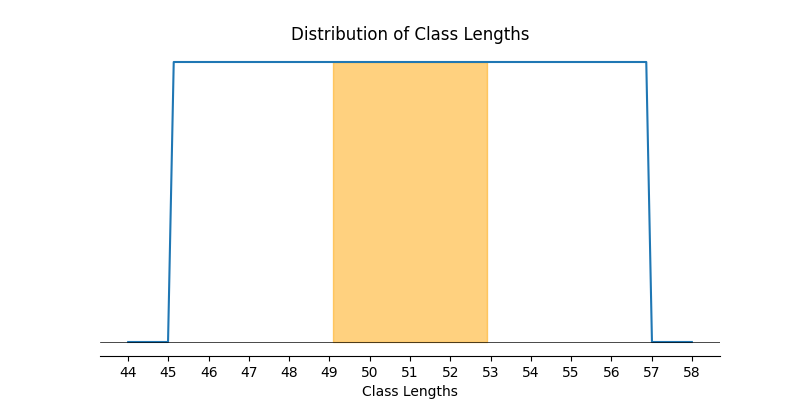
With drawing the figure we notice there is no y-axis. However, we do know the total area under the figure must be equal to 1 so we can set up the following relationship \[A_{\text{fullbox}}=L_{\text{fullbox}}*W_{\text{fullbox}}\] where \( A_{\text{fullbox}}\) represents the area of the uniform distribution (which we know is 1 since this is a density function), \( L_{\text{fullbox}}\) represents the length of the uniform distribution (which we see is 12 by performing the subtraction \(57-45=12\)), and \( W_{\text{fullbox}}\) represents the width of the uniform distribution. Then doing a little algebra we can solve for the width \( W_{\text{fullbox}}\) as follows \[ A_{\text{fullbox}}=L_{\text{fullbox}}*W_{\text{fullbox}} \to 1 = 12*W_{\text{fullbox}}\] which reduces to (after dividing by 12 on both sides) \[ W_{\text{fullbox}} = \cfrac{1}{12} \approx 0.08\overline{3}\]

Since we now know the width of our probability distribution, we can get a much better picture of what area we want to find with all the appropriate labeling

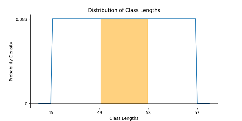
Now finding the solution for the problem we simply apply geometry to find the area which will be length times width. This gives us \(A=4*0.08\overline{3}\approx 0.33\overline{3}\). So the probability for a class time lasting between 49 mins and 53 mins is found to be about 33.3%.